Bringing Autodiff to Geometry
Published May 25, 2026 · 6 min read
Automatic differentiation (autodiff) computes exact derivatives by tracing a computation graph and applying the chain rule - no symbolic algebra, no finite differences. It is the technique behind modern ML frameworks like JAX, PyTorch, and TensorFlow.
Geomatic brings autodiff to a geometric setting, running entirely in your browser. Distances, angles, and areas become differentiable expressions whose gradients can be visualized and acted on interactively. Autodiff in visual domain can illuminate problems that are hard to reason through otherwise. The gradient of an angle, for instance, has a beautiful interpretation - it always points toward the circumcenter - which becomes immediately clear when drawn. See Gradient of an Angle.
Things you can do with autodiff
\backprop
\backprop runs reverse-mode autodiff: given a scalar loss, it computes the gradient with respect to every named parameter in the computation graph. One then takes a gradient descent step to reduce the loss and repeats until convergence. Some examples that use backprop:
- Fermat Point of a Triangle - find the point that minimizes total distance to all three vertices using iterated
\backpropand gradient steps. - Finding Square Root with Gradient Descent - frame square-root as a least-squares problem and converge to the answer purely through backprop.
\tangent
\tangent computes the tangent to a curve or function at a given point using autodiff, returning the slope or tangent vector directly. Some examples that use tangent:
- Plotting Functions and Tangents - plot and attach a tangent line that moves as you slide along the curve.
- Newton-Raphson method visualized
vector-field
vector-field visualizes a vector field on a grid. Supply a scalar function and Geomatic differentiates it automatically to produce the gradient field. You can also provide a vector field directly by defining an function, giving full control over direction and magnitude at every grid point.
- Vector Field I: Gradient of a Scalar Function - visualize the gradient field of a parametric scalar function and watch it transform as you change the parameter.
- Vector Field II: Directly Defined Vectors - define a rotational field by hand and explore how parameters shape it.
\minimize
\minimize wraps the backprop-and-step loop into a single command, running gradient descent until convergence. Draw the geometry, declare a loss, and let \minimize find the answer - no manual iteration needed.
- Using Optimization to Set Up a Problem Quickly - place a point inside a square at prescribed distances from three vertices, solved directly with
\minimize.
Differentiating through user-defined functions
What makes Geomatic's autodiff especially powerful is that it works through user-defined extension functions - functions you write yourself and load into the system. The engine traces the computation graph through custom code exactly as it does for built-in functions. Any custom geometric or analytic construction becomes immediately differentiable. This opens the door to problems that built-in primitives alone cannot express.
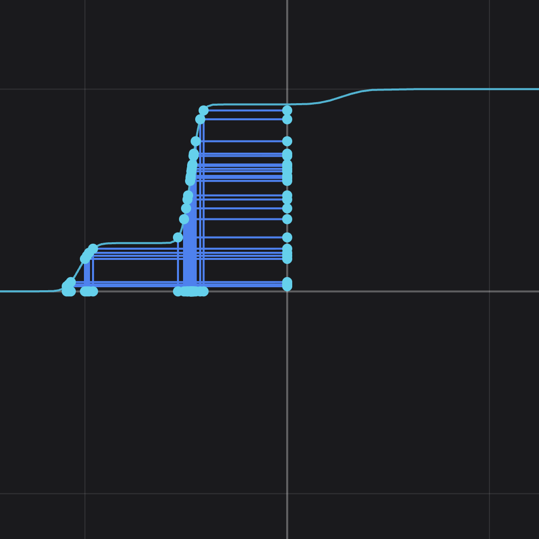
As a fun exercise, use the \normalizing-flow command followed by \minimize loss n to train a toy example of normalizing flows using Gaussian CDFs in the Geomatic editor. You will have to tweak the learning-rate a couple of times to make it work. Here is what I was able to achieve after a few hundreds of steps of training: